What the heck is a Chu space? And whatever it is, does it really belong with all the rich mathematical structures we know and love?

Say you have some stuff. What can you do with it?

Maybe it’s made of little pieces, and you can do a different thing with each little piece.

But maybe the pieces are structured in a certain way, and you aren’t allowed to do anything that would break this structure.

A Chu space is a versatile way of formalizing anything like that!

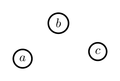
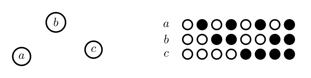
To represent something in a Chu space, we’ll put the names of our pieces on the left. How about the rules? For a Chu space, the rules are about allowed ways to color our pieces. To represent these rules, we can simply make columns showing all the allowed ways we can color our pieces (just get rid of any columns that break the rules). Here’s what a basic 3-element set (pictured on the left) looks like as a Chu space:

It doesn’t have any sort of structure, so we show that by allowing all the possible colorings (with two colors). Chu spaces that don’t have any rules (i.e. all colorings are allowed) are equivalent to sets.

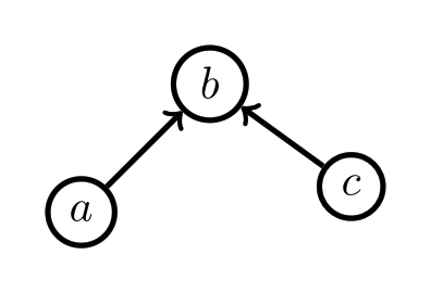
What about the one with the arrows from above? How can we make an arrow into a coloring rule? One way we could do it is by stipulating that if there’s an arrow $x \rightarrow y$ , we’ll make a rule that if $x$ is colored black, then $y$ has to be colored black too, where $x$ and $y$ can stand in for any of the pieces. Here’s what that Chu space looks like:

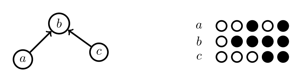
Spend a minute looking at the picture until you’re convinced that our coloring rule is obeyed for every arrow on the left side of the picture. Any Chu space that has this kind of arrow rule has the structure of a poset.

There and back again

If we have two Chu spaces, say $A$ and $B$ , what sort of maps should we be able to make between them?

We’d like to be able to map the pieces of $A$ to the pieces of $B$ . So this part of our map will just be a normal function between sets:

$f:A_{\textsf{pieces}}\rightarrow B_{\textsf{pieces}}$

But we also want our maps to respect the rules of $A$ as it maps to $B$ . How can we check this?

Let’s think through how we would be able to tell if a potential map did break the rules. The map will take pieces of $A$ to pieces of $B$ , so let’s look at the pieces of $B$ that got mapped onto, i.e. $f(A_{\textsf{pieces}})$ . It will help if we have a concrete example in mind, so let’s consider a potential map that we think should break the rules: one that breaks the arrow structure of a poset by breaking it up into a mere set. For simplicity, we’ll just have the pieces map $f$ take pieces to pieces with the same label.

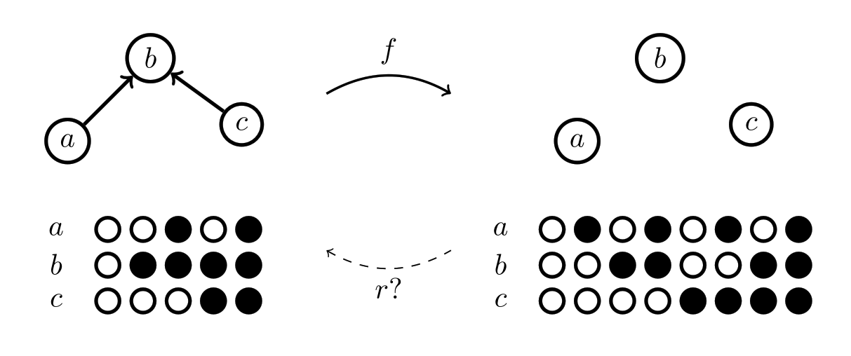
We can see now that if this potential map breaks the rules, it must be because some of the colorings for $f(A_{\textsf{pieces}})$ are invalid. Specifically, the colorings highlighted in red:

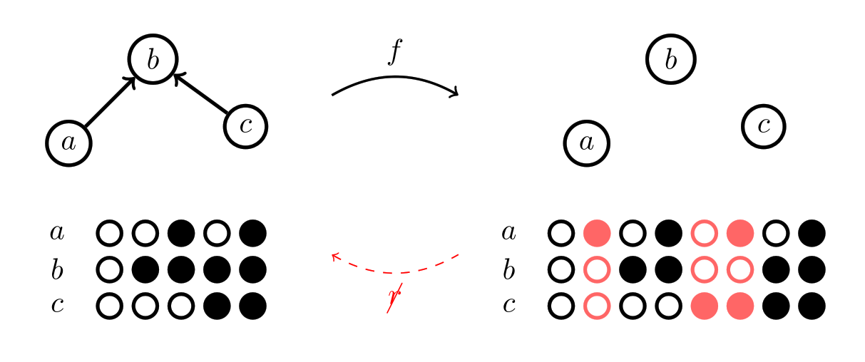
The problem with these colorings is that there are no colorings in the original space for them to correspond to; so they must break one of the rules of the original space. So for a map that does follow the rules, we’ll want to make sure every coloring in $B$ has a corresponding coloring in $A$ . This will be another function between sets, this time going backwards between the sets of colorings:

$r:B_{\textsf{colorings}}\rightarrow A_{\textsf{colorings}}$

Now let’s look at an example of what we expect should be a legit map between Chu spaces.

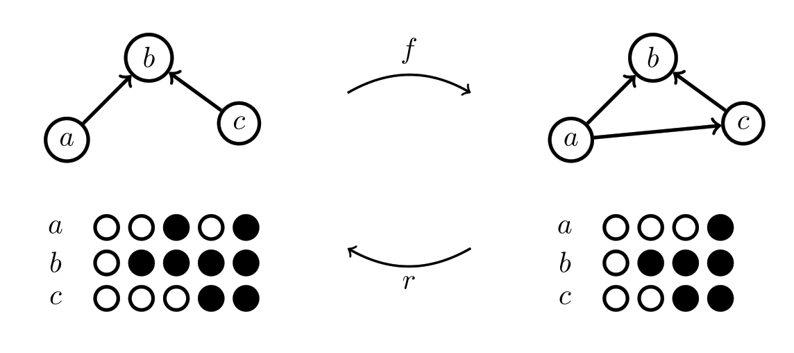
Again, we are just mapping pieces to pieces with the same labels. This map is ok because even though $B$ has some additional structure, it respects all of the structure from $A$ .

The last part we need to define a map between Chu spaces is to determine exactly what it means for colorings of $B$ to have a corresponding coloring in $A$ . For a given piece $x$ , and a given coloring $s$ , we have a function that gives us the color of $x$ using the coloring $s$ :

$\mathsf{Color}_A:A_{\mathsf{Pieces}}\times A_{\mathsf{Colorings}} \rightarrow \mathsf{Palette}$

We want to make sure that if we have a coloring $s$ from $B$ , that it gets taken back to a compatible coloring in $A$ . The coloring it gets taken back to is $r(s)$ , and we can check it’s color on any piece $p$ from $A$ with $\mathsf{Color}_A(p, r(s))$ .

What do we want this to be the same as? It should be the same as the our coloring $s$ from $B$ on all the pieces that $f$ maps onto! We can check these colors with $\mathsf{Color}_B(f(p), s)$ . And so, we can finish our notion of a Chu map by making sure that for all the pieces $p$ of $A$ , and for all colorings $s$ of $B$ , that the following equation holds:

$\mathsf{Color}_B(f(p), s)=\mathsf{Color}_A(p, r(s))$

Thus, a map between Chu spaces is made of any two functions $f$ and $r$ which satisfy the above equation.

Basic concepts

In order to talk about Chu spaces more easily, let’s define some terminology.

The set of “pieces” is known as the carrier, and each “piece” is called a point. These points index the rows. Likewise, each “coloring” (i.e. column) is indexed by a state, and the set of states is called the cocarrier. Each point-state pair has a “color” which is a value taken from the alphabet (or “palette”). For a Chu space $C$ with point $p$ and state $s$ , we’ll denote this value by $C\langle p,s \rangle$ .

A Chu transform is a map between two Chu spaces: $t: A\rightarrow B$ . It is composed of two functions, the forward function $f$ from the carrier of $A$ to the carrier of $B$ , and the reverse function r from the cocarrier $B$ to the cocarrier of $A$ . These must satisfy the Chu condition in order for this $t$ to be a Chu transform: For every point $p_A$ of $A$ and every state $s_B$ of $B$ ,

$B\langle f(p_A), s_B\rangle = A\langle p_A, r(s_B)\rangle$

We say a Chu space is separable if all the rows are unique. It’s extensional if all the columns are unique, and biextensional if both the rows and the columns are unique. We can make any Chu space biextensional simply by striking out any duplicate rows and columns. This is known as the biextensional collapse. Any two Chu spaces with the same biextensional collapse are biextensionally equivalent. It’s very common in applications to only consider things up to biextensional equivalence.

Chu spaces with Chu transforms form a category. This category is typically called $\mathbf{Chu}_{|\Sigma|}$ , where $\Sigma$ is the alphabet.

Representation

Lots of categories are fully embedded into $\mathbf{Chu}_2$ , and even more if we allow arbitrarily many colors. Let’s look at some examples so we can get a better feel for how we can represent different kinds of rules with coloring rules.

For a topological space, the pieces will be all the points. The allowed colorings will be exactly the ones where the pieces colored white make up an open set, and the pieces colored black make up a closed set. It’s then easy to how the Chu transform gives us exactly continuous functions between topological spaces!

This example also motivates why Chu spaces are called spaces: for any two color Chu space, we can think of each column representing a generalized open set, containing the white colored points.

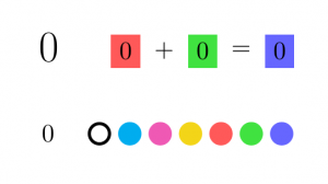
If we use more colors, we can embed any category of algebraic objects fully and faithfully into Chu! In other words, Chu can represent any algebraic category. To see how this works, let’s see how we can represent any group. The points will be the elements of the group. We’ll need 8 colors, which we’ll think of as being the 8 combinations of red, green, and blue. We’ll think of each relation $rg=b$ as having the $r$ slot colored red, the $g$ spot colored green, and the $b$ spot colored blue. Only colorings which have at least one element in the right color slot for ALL the relations of the group are allowed. We need 8 colors to represent the possibility of the same element appearing in multiple slots. For example, with the zero group, 0 appears in every slot for every relation, so the 0 row will have all the colors which have at least red, green, or blue “turned on”:

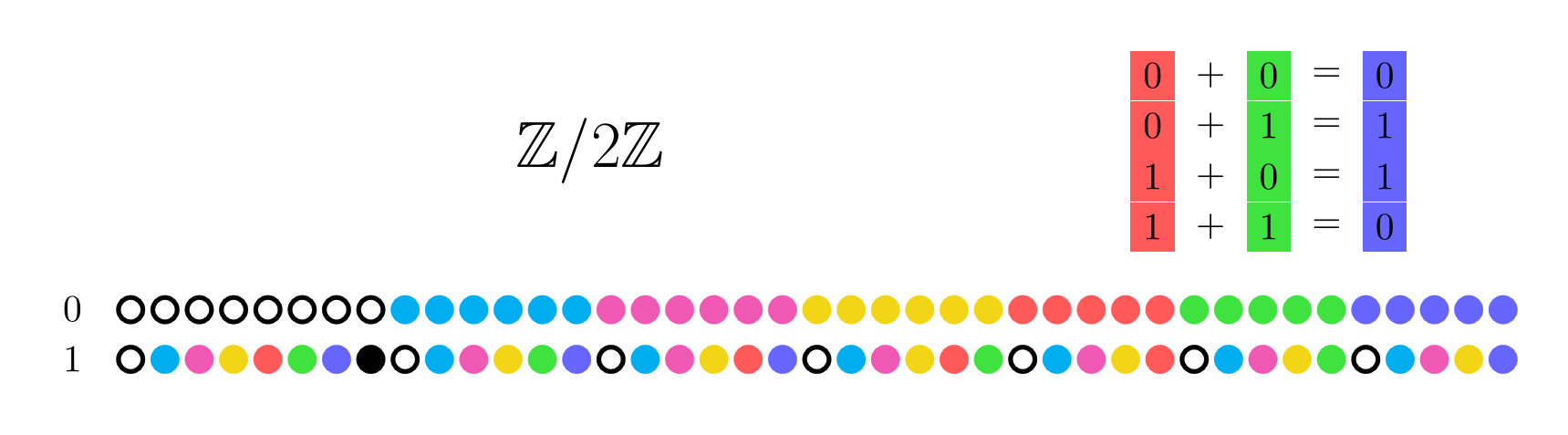
This is not an economical representation. Even for just the cyclic group of order 2, we need lots of rules (41, to be exact)¹.

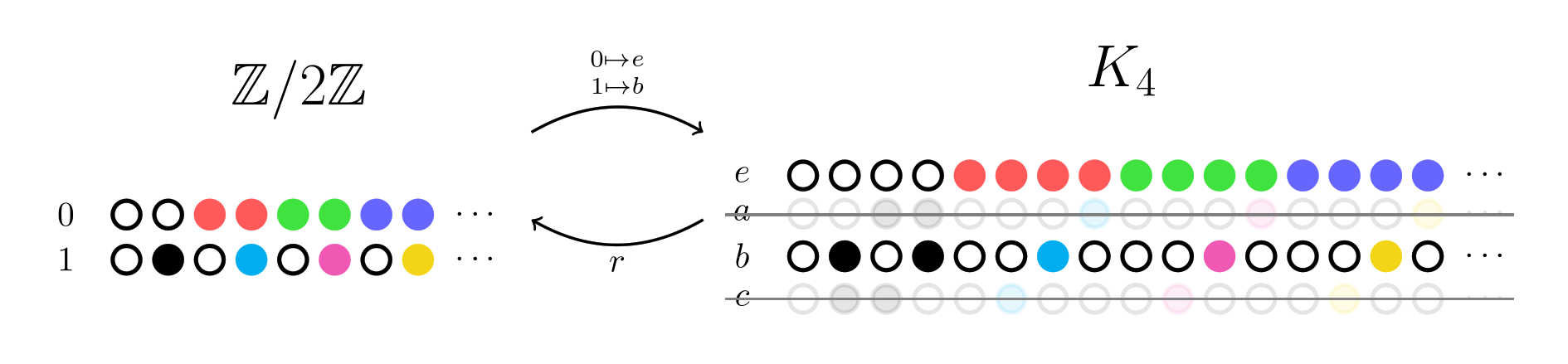
The Klein 4-group requires 1045 columns under this representation! So the following pictures will be truncated, so that we can see the essential idea without being overwhelmed. Let’s consider a potential Chu transform between $\mathbb Z / 2\mathbb Z$ and $K_4$ with this representation:

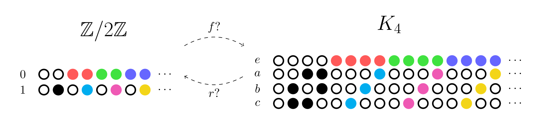
The forward map $f$ is almost like a question. It chooses which rows 0 and 1 should correspond to (say $e$ and $b$ respectively), and asks if this is an allowed transformation.

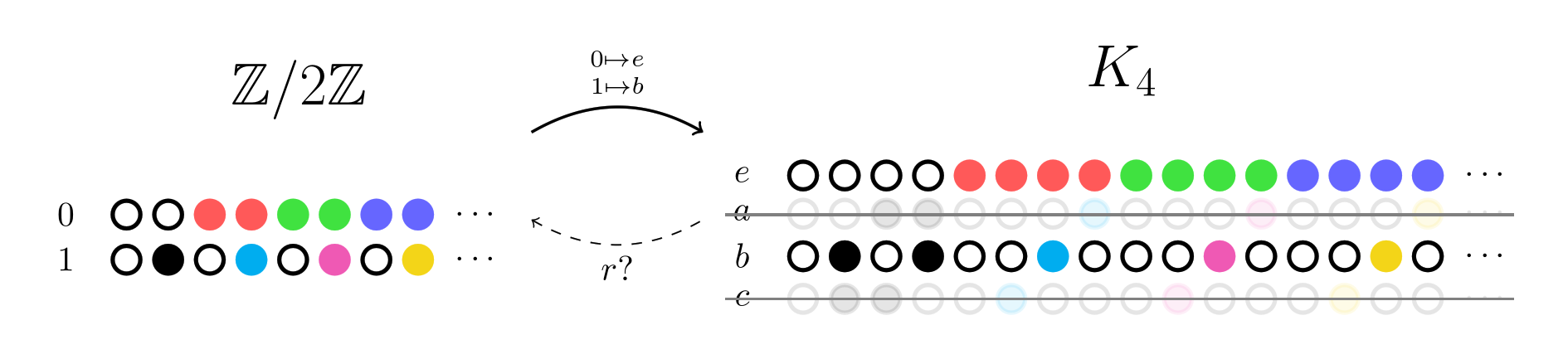
The reverse map $r$ responds by finding the representative of each column from $K_4$ . E.g. the 2nd column of $K_4$ must be mapped to the 2nd column of $\mathbb Z / 2\mathbb Z$ . If it can’t find such a map, we can think of this as an answer in the negative.

Let’s look at another example where the reverse map is slightly more interesting. We expect there to be a group homomorphism from $K_4$ to $\mathbb Z / 2 \mathbb Z$ , so let’s check that this is the case for the Chu spaces as well. (We’ll show a different subset of the columns of $K_4$ in this example.)

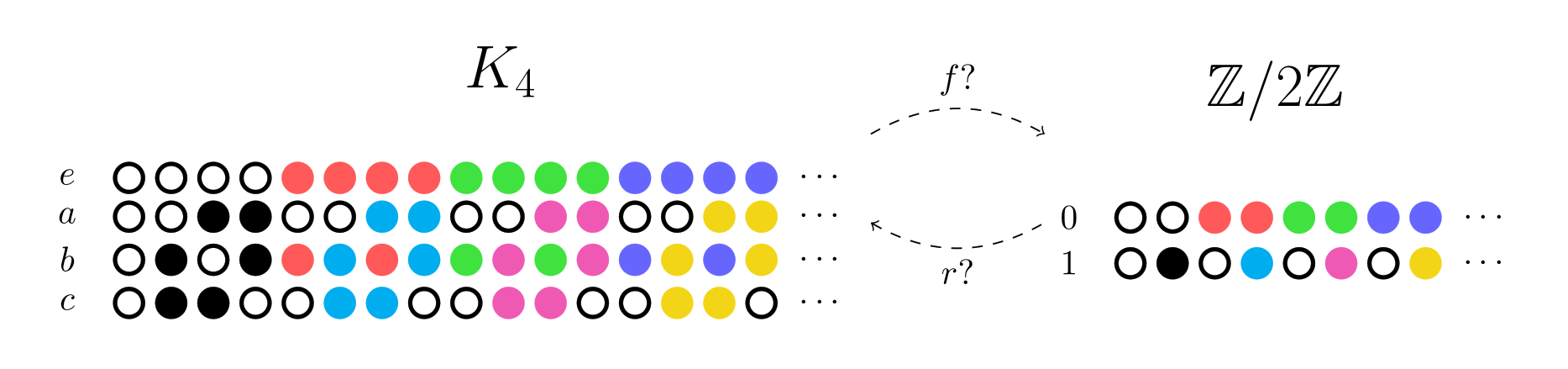
Again, we’ll choose a forward map, this time taking $e$ and $b$ to 0, and $a$ and $c$ to 1. The reverse map then verifies that the group structure is satisfied, by looking for a column of $K_4$ for every column of $\mathbb Z / 2 \mathbb Z$ .

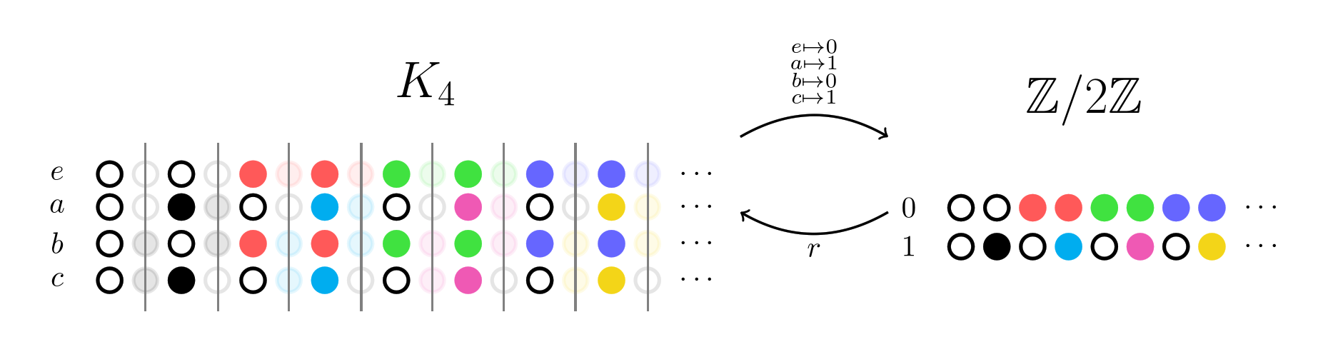
Notice how the alternating color columns get chosen by $r$ . This is mandated by the Chu condition, given that $f$ maps its rows in an alternating pattern.

Notice also how we didn’t need to add anything else to properly represent group axioms, such as the fact that every group has an identity. Instead, this is encoded implicitly: the identity row will be the only row that doesn’t contain any black, so the Chu condition thus ensures it must always be mapped to the identity of another group represented this way. By simply specifying all the relations that are allowed, we’ve implicitly specified the entire structure! This seemingly innocuous observation is at the heart of the celebrated Yoneda lemma.

Yoneda

The Yoneda lemma could rightly be called “the fundamental theorem of category theory”. While fundamentally a simple result, it is notoriously difficult to understand. An important corollary is the Yoneda embedding (and also the co-Yoneda embedding). There is an analog of the Yoneda embedding for Chu spaces which can be proved directly (without the Yoneda lemma) and which is conceptually simpler! I’ll prove that version in full here, since I found it enlightening to see exactly how it works.

Theorem: Every small² category $C$ embeds fully into $\mathbf{Chu}_{|C|}$ .
Proof: The embedding works by defining a functor $Y:C\rightarrow\mathbf{Chu}_{|C|}$ . For each object $c\in C$ , $Y$ takes this object to the Chu space where the points are all the arrows into $c$ , and the states are all the arrows out of $c$ . Here’s an example category $E$ :

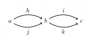
And here are the three Chu spaces that $Y$ makes out of $E$ (one for each object), along with some of the induced Chu transforms (which will be defined below):

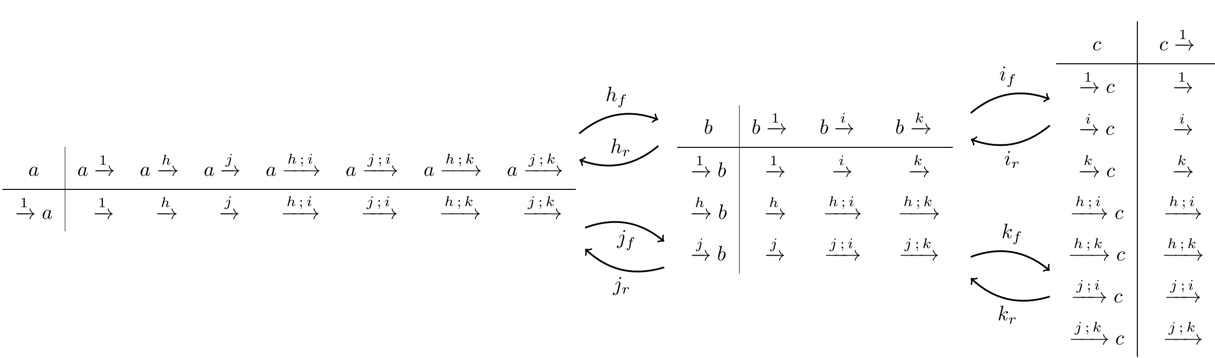
In any case, $Y(c)$ is separable because the identity column will be different for each distinct point (i.e. incoming morphism). Similarly, it is extensional since the identity row will be different for each distinct state (i.e. outgoing morphism). So $Y(C)$ is biextensional.

Now consider a morphism $g: c\rightarrow d$ in $C$ . $Y(g)$ must of course be a Chu transform, hence is composed of a pair of functions $(g_f, g_r)$ between the carriers and cocarriers of $Y(c)$ and $Y(d)$ . Specifically, $g_f$ will take a point $p$ of $Y(c)$ (i.e. incoming morphism to $c$ ) to a point of $Y(d)$ (an incoming morphism to $d$ ) defined by $g_f(p)=p \,; g$ . Similarly, $g_r$ will take a state $s$ of $Y(d)$ to a state of $Y(c)$ via $g_r(s)= g \,; s$ . This satisfies the Chu condition since function composition is associative:

$Y(d)\langle g_f(p), s \rangle = g_f(p) \,; s = (p \,; g) \,; s = p \,; (g \,; s) = p \,; g_r(s) = Y(c)\langle p, g_r(s) \rangle$

This functor is faithful, which means that it keeps morphisms distinct: if $g, h: c\rightarrow d$ are distinct morphisms, then $Y(g)$ and $Y(h)$ are also distinct. We can see this by checking the values of $g_f(1_c) = 1_c\,; g = g$ and $h_f(1_c)=h$ .

And finally, this functor is full, which means that every Chu transform between the Chu spaces of $Y(C)$ comes from a morphism of $C$ . We can see this by taking an arbitrary Chu transform $(f, r) : Y(c) \rightarrow Y(d)$ . From the Chu condition $Y(d)\langle f(1_c), 1_d\rangle = Y(c)\langle 1_c, r(1_d)\rangle$ , which implies that $f(1_c)=r(1_d)$ . By construction, this is a morphism $m$ of $C$ starting at $c$ and ending at $d$ , i.e $m:c\rightarrow d$ . Again by the Chu condition, $f(p) = Y(d)\langle f(p), 1_d\rangle = Y(c)\langle p, r(1_d)\rangle = p \,; m$ . Similarly, $m \,; s = \langle f(1_c), s\rangle = \langle 1_c, r(s)\rangle = r(s)$ . Thus, $f$ is exactly $m_f$ , and $r$ is exactly $m_r$ as given by $Y(m)$ . This means our transform was just $Y(m)$ . QED

Having a full and faithful embedding into $\mathbf{Chu}_{|C|}$ means that our category $C$ is represented by $\mathbf{Chu}_{|C|}$ . This is quite similar to how groups can be represented by vector spaces!

Also notice how we needed three things to make this work: identity morphisms for each object, composition of morphisms, and associativity of composition. These are exactly the requirements for a category! I think this explains why categories are such a fruitful abstraction: it has exactly what we need to make the Yoneda embedding work, and no more.

Final thoughts

Hopefully I’ve convinced you that Chu spaces are indeed a mathematical abstraction worth knowing. I appreciate in particular how they provide such a concrete way of understanding otherwise slippery things.

This post just scratches the surface of what you can do with Chu spaces. Now that I’ve laid out the basics, I plan to continue with another post about how Chu spaces relate to linear logic, cartesian frames, Fourier transforms, and more!

Most of the stuff in this post can be found in Pratt’s Coimbra paper. There aren’t many distinct introductions to Chu spaces so I thought it was worth retreading this ground from a somewhat different perspective.

Special thanks to Evan Hubinger for encouraging me to write this up, and to Nisan Stiennon for his helpful feedback!

Footnotes

[1]: For $\mathbb Z / 2 \mathbb Z$ , there are four relations of the form $r + g = b$ . Let’s start with 0 + 0 = 0. To cover this relation, we must turn on either the red, green, or blue light for 0. So the 0 row will never be colored black. If we color 0 white, then we’ve covered every relation, since every relation has 0 in either the r, g, or b slot. On the other hand, if we colored 0 green, then we would need to turn on either the blue or the green light for 1 in order to cover the second equation 0 + 1 = 1. If we turned on the blue light for 1, then the third equation 1 + 0 = 1 would be covered already, but the fourth equation 1 + 1 = 0 won’t. We’ll have to turn on either the red or the green light for 1 in order to cover the fourth equation. Here’s the code I used to calculate these.

[2]: A small category is simply one where the objects and morphisms are both sets. They could even be uncountable sets! A category that isn’t small is $\mathbf{Set}$ . That’s because the objects of this category are all sets, and we can’t have the set of all sets lest we run into Russell’s paradox.

Chu are you?

Published by adele on 2021-11-052021-11-05

There and back again

Basic concepts

Representation

Yoneda

Final thoughts

Footnotes

0 Comments

Leave a Reply Cancel reply

logic

Visual Linear Logic

math

Sperner’s lemma

Chu are you?

Published by adele on 2021-11-052021-11-05

There and back again

Basic concepts

Representation

Yoneda

Final thoughts

Footnotes

0 Comments

Leave a Reply Cancel reply

Related Posts

logic

Visual Linear Logic

math

Sperner’s lemma