Visual Linear Logic

What even is logic anyway?

Logic is about what patterns of thought are valid. There are different kinds of logic for thinking about different kinds of things. Classical logic is for thinking about truth. Intuitionistic logic is for thinking about proofs. And linear logic is for thinking about resources!

What does that actually mean? Well, resources are basically ordinary sorts of things that are usable, and typically are limited. So we’ll understand linear logic just by trying to understand what sort of things we can do with things. Let’s see how it works!

Instead of using the typical notation for logic, we’re going to use an experimental visual notation based off of Charles Sanders Peirce’s Alpha diagrams.

Charles Sanders Peirce was an American mathematician and philosopher who independently discovered first order logic (introducing the quantifier symbols and commonly used today). In his later years, he felt strongly that logic notation should be made to correspond as closely as possible to the ideas they represented (i.e. be iconic), and developed his Alpha diagram system to achieve this. The visual diagrams used here are my attempt to continue his vision by developing an iconic notation for modern logics.

My hope is that making this visual will make linear logic less intimidating, and more accessible to a wider audience. I also find it easier and more fun to think about! Plus, the visual notation might lead to some creative insights.

To help connect this to the standard notation for linear logic, I’ll caption most of the images with the standard notation for them. Don’t worry if you don’t understand this, it’s just there to help you connect this with the existing stuff about linear logic.

Thanks to everyone on Twitter who gave their feedback on this!

Basic Things

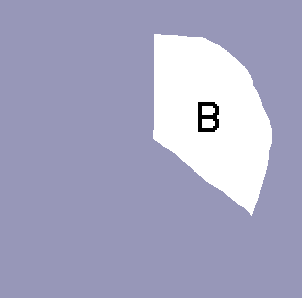
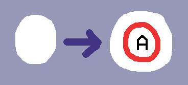
The most basic thing we can do with something is to have it. When we have something, we’ll write its name in a white bubble like this:

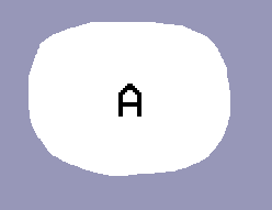
This name could refer to a particular resource, or even a different bubble (or nested bubbles), or combinations of other items. Just like a variable identifier!

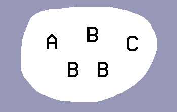
Of course, we may have multiple things. Perhaps even multiples of the same thing. To denote this, we’ll simply write the name of every single thing we have in our white bubble:

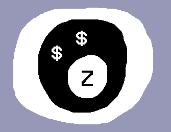
More interestingly, we may also have things that can exchange things. We can call these contracts, trades, or ‘what-ifs’. For example, we might have a contract allowing us to trade two dollars for item Z. We’ll draw this contract like this:

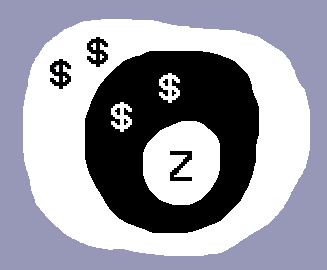
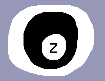
If we actually have two dollars with this contract, we would be able to buy item Z. That looks like this:

Notice that the transfer actually happens in two steps. First we pony up the cash, resulting in a fulfilled contract which promises us Z:

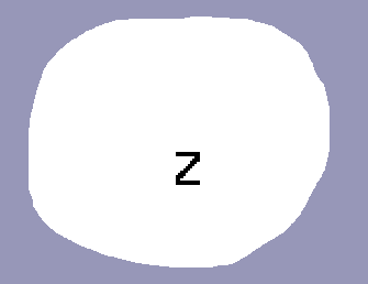
Now that the contract is fulfilled, we can actually get Z:

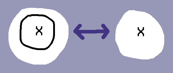
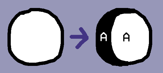
We can always switch back-and-forth between an item, and a fulfilled contract for that item. In our drawings, this looks like adding or removing a black loop as we please, around whatever we want:

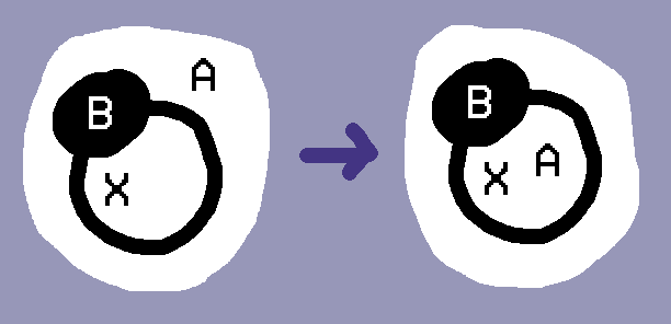
Another thing we can do if we have a contract along with something else is to put that something else on the other side of the contract. That might not seem particularly useful, but it’s important because it allows us to reason about how things we could get would interact with the things we already have:

We’re also free to take out “loans”. First, we can set up a dummy contract by making a black loop around nothing. Then, we can put the same thing on either end of the contract, once in white and once in black, to get something like this:

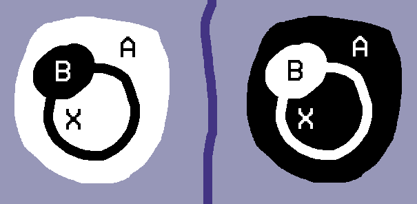
All it means is that if we had A, then we’d have A. But it helps us see an important thing, which is that in some sense, the white text and the black text are opposites. In fact, to get the opposite of multiple things, we can invert the entire image:

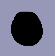
This raises the question of what a solid black bubble means. A white bubble is just nothing — a free region where we can have things and do stuff. That white bubble is the emptiness in which we live! So a black bubble is a fulfilled contract without the other side, no future possible. Death.

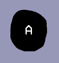
In general, the inverted bubble can be thought of as the most emphatic denial of what the original bubble signifies. So if we just have A, the inverted bubble we’ll call Not A. Or more emphatically: “Not A! Or else…” It’s not outright impossible that you might still have A, it’s more like a threat of what will happen to you if you are unlucky enough to have both.

There’s one more situation possible with the stuff introduced so far, a contract within a contract. Say we had a contract where if we provided A, we would get another contract which would give us C for B:

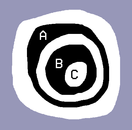
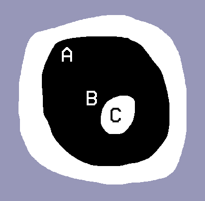
We’re always allowed to reconceptualize it as a single contract where we trade A and B to get C. We can think of this as removing a white loop:

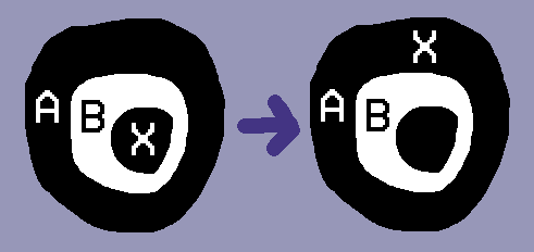
But if the outer contract lets us pay A to get B and not X, then it would seem that we should be able to do something similar despite the presence of B. So we also have a rule that lets us pull the not X out into another black region:

To summarize the rules we’ve developed, we can add and remove black and white loops at will (doesn’t matter what’s inside the loop):

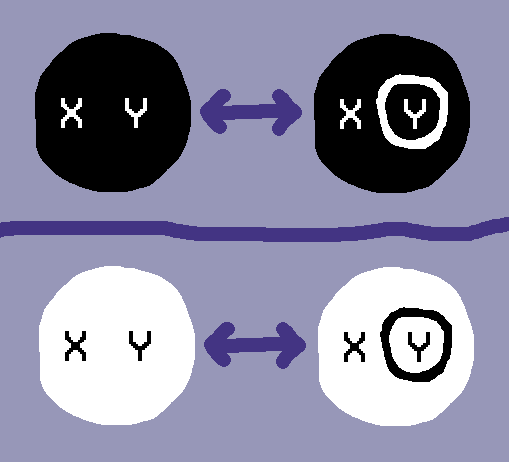
And we can push things into white, and pull things out to black:

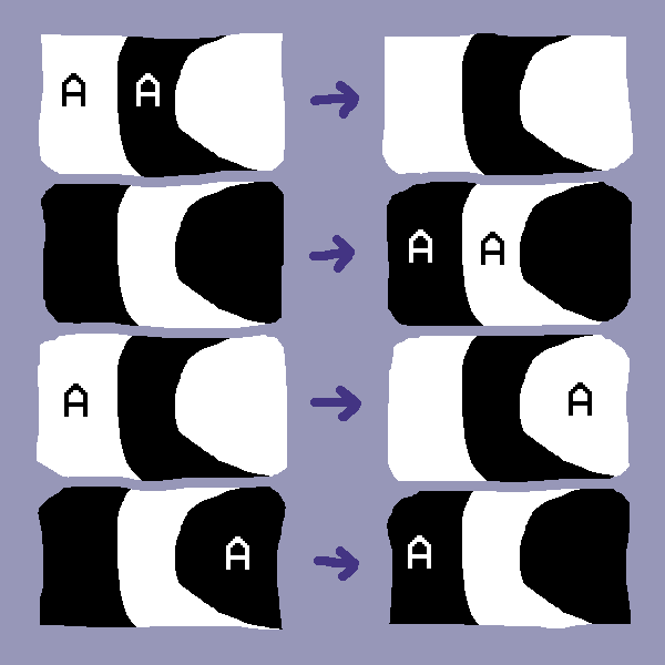
Notice how each rule has a reversed counterpart, where the colors are inverted, and the direction the indigo arrow points is flipped. This is something that every rule in linear logic has: a reversal.

Now let’s show off this visual calculus! Let’s show that if we have a contract where we can trade A for B, and another contract where we can trade B for C, then we can combine these into a contract letting us trade A for C.

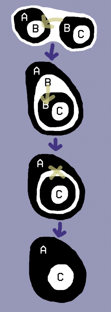
The diagram calculus in this section is a modified version of the one discovered by Brady and Trimble in https://core.ac.uk/download/pdf/82545173.pdf

Choices and Contingencies

Sometimes we might have a choice on what to do with a certain bubble. Sure, we could just choose one, but what if we wanted to trade the choice itself?

To handle this situation, we’ll introduce a new kind of bubble called a choice bubble. These bubbles are sectioned by blue lines like this:

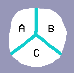
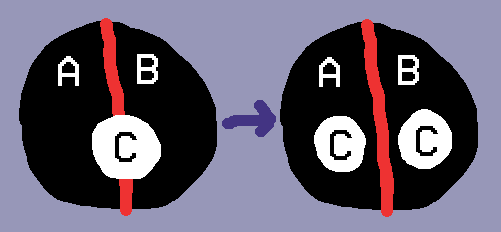
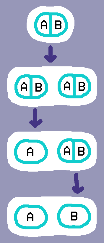
Each section is its own bubble, though things aren’t allowed to pass through these until we choose one of them. Once we choose any section, the rest of the bubble collapses, and that section is all that remains:

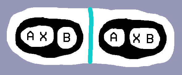
To create a choice bubble, we can always just duplicate an existing bubble, i.e. put the contents of the bubble into all sections of a choice bubble:

So if we wanted to represent the choice itself presented at the beginning of this section, we could draw it like this:

Blue lines don’t always split bubbles cleanly, sometimes it only splits the outer bubble:

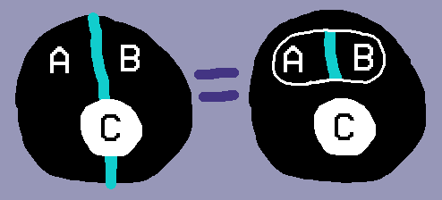
You can see above that it means exactly the same thing as if all the stuff in the outer bubble was split in its own bubble. It doesn’t matter if the colors of the bubbles are white or black, it works the same way in any case.

The reason we allow this notation is so that our next rule is more intuitive. If two bubbles on different sides of a blue line are identical, we can pinch them together:

This rule works on bubbles of any color, of course! It makes sense because we can think of it as saying that if we have a choice between two contracts that give us the same thing C, then we can think of it as a single contract that lets us choose between the two different costs.

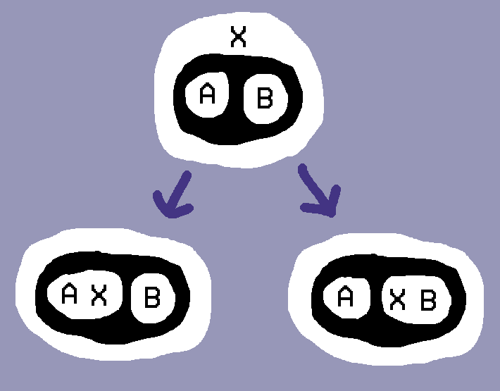
As we might expect by now, there’s an opposite to a choice bubble. If our choice bubble is the one on the left, its opposite will be the bubble on the right:

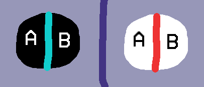
Since it’s the opposite of a choice bubble, we call this kind of bubble a contingency bubble. But what does that actually mean? The rule for creating one will be the reverse of the rule for popping a choice one. So this means that we can make this kind of bubble from an existing bubble by putting the existing bubble in one section, and the other sections can have arbitrary stuff in them!

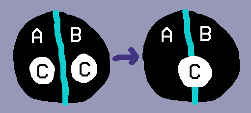
On the other hand, we can only get rid of this bubble if all the sections have the same thing in them, then we can just collapse it all into just one section:

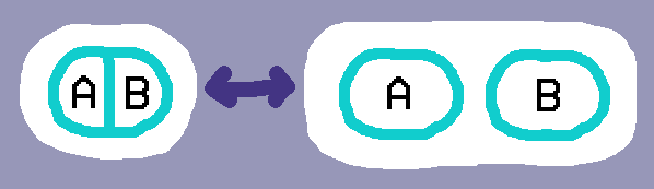
And finally, we can unpinch bubbles:

With either of these kinds of bubbles, it’s important to remember that you can’t move stuff through them like the white and black bubbles (though you are free to move the entire bubble if it lies in a white or black bubble).

Of course!

Some resources are actually unlimited! A digital song is a good example: you can copy and share it with as many people as you like (or at least within legal and physical limits), while still keeping your own copy in pristine condition. So far, we don’t have a way of representing this kind of resource.

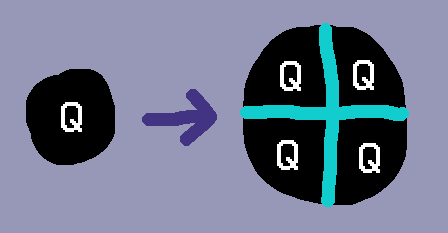
To say that something is available in any amount, we’ll put a blue loop around it:

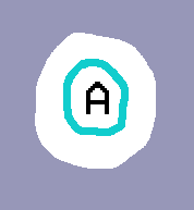
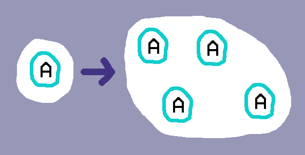
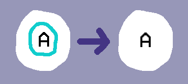
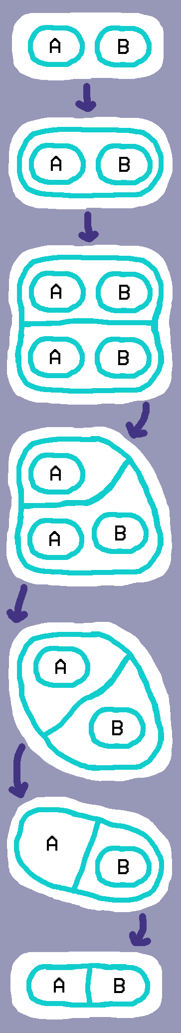
We’ll call this an unlimited bubble. We can replace an unlimited bubble with any number of copies of itself:

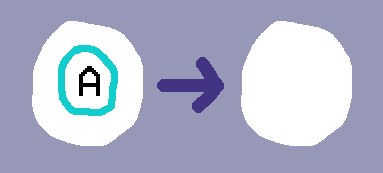
Importantly, we can also delete the entire bubble (technically included in the last rule by replacing it with zero copies of itself):

And finally, we can remove the loop. This lets us actually use the contents, since we can’t pass things through the loop itself.

To create a blue loop, we can put a blue loop around any number of unlimited bubbles lying in the same white region. This makes intuitive sense, since if we have an unlimited number of a bunch of things, we have an unlimited number of all of them together:

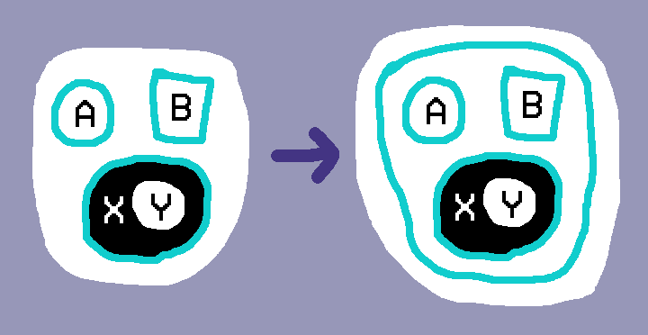
Importantly, this includes putting a blue loop around an empty white region, which allows us to use tautologies an unlimited number of times!

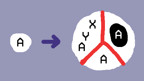
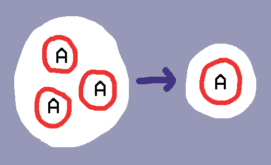
Of course, unlimited bubbles have an opposite, called a maybe bubble, which have a red loop. These follow the reverse of the unlimited bubble rules.

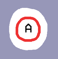
We can put a red loop around any bubble.

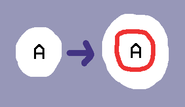
We can make a maybe bubble with whatever we want in it.

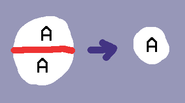
We can collapse a bunch of copies of maybe bubbles into one.

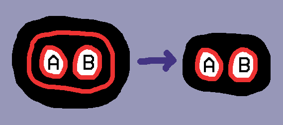
We can remove a red loop if everything in it is a maybe bubble lying in a black region.

They may not seem like much, but these two new bubble types add a lot of power to our logic. For example, we now are able to fully embed classical logic into our linear logic.

Example proof

Let’s try this visual notation out to see how we can use it to prove a classic linear logic identity! This identity has to do with unlimited choice bubbles:

The blue line splitting choice bubbles and the blue loop of unlimited bubbles are the same color for a reason, it’s to make this identity look visually intuitive! Let’s see how we prove this:

Proofs can be animated! The following gif shows that if we can already prove the relation shown on the first frame, then we can prove it with a blue loop around it, except for around the red looped parts. This is an instance of Girard’s promotion rule.

Next steps

I’ve also extended this for first order logic, which I’ll write about in an upcoming post! I additionally have some ideas for extending this visual notation for dependent type theory, which I’m really excited about!!

I believe it’s possible to modify this notation for intuitionistic linear logic simply by removing the rule that lets you remove a white loop, and only allow blue on white and red on black.

It would also be super awesome to make this into an interactive program so you can play with it. I’m hoping that it won’t be too much trouble to use penrose.ink for this purpose.

References

Linear Logic

nLab — Linear Logic

Linear Logic Prover by Tamura

Linear Logic: its Syntax and Semantics by Girard

Linear Logic for Linguists by Crouch and van Genabith

Linear Logic for Constructive Mathematics by Shulman

A Taste of Linear Logic by Wadler

Existential Graphs

Peirce’s Tutorial on Existential Graphs by Sowa

A categorical Interpretation of C.S. Peirce’s
Propositional Logic Alpha by Brady and Trimble